If your Power BI report is slow, your DAX is convoluted, or your filters aren’t working as expected — the problem is almost always the data model, not the formula. The star schema is the single most important design decision you’ll make. Get it right, and DAX becomes almost effortless. Get it wrong, and no amount of formula skill will save you.
Fact tables vs. dimension tables
A well-modeled Power BI dataset has two types of tables:
Fact tables record events. Each row is a transaction, an order, a click, a measurement. They’re narrow (few columns) and long (many rows), and they consist mostly of:
- Foreign keys — pointers to dimension tables (
ProductKey,CustomerKey,DateKey) - Measures — numeric values you aggregate (
Revenue,Quantity,Cost)
Dimension tables describe the entities involved. Each row is a unique entity, and the table is wide (many descriptive columns):
Product— ProductKey, Name, Category, Brand, Color, ListPriceCustomer— CustomerKey, Name, Segment, Country, CityDate— Date, Year, Quarter, Month, Weekday
The fact table holds “what happened,” the dimension tables hold “who, what, when, where.” This separation is the foundation of the star schema.
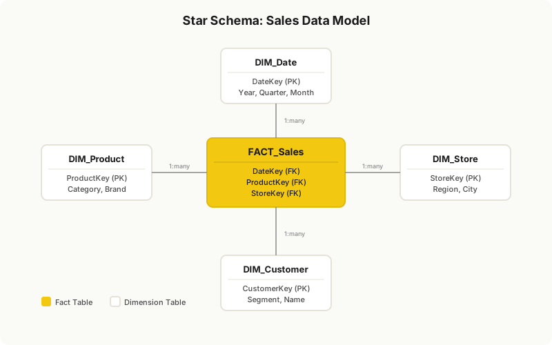
In the diagram above, FACT_Sales sits at the center with foreign keys pointing outward to four dimension tables. Each dimension connects to the fact table with a one-to-many relationship — the “star” pattern that gives this design its name.
Why not just use one big table?
Many beginners load a single flat Excel sheet with every column. It works for a 50-row prototype, but at scale:
- Filters become slow — the engine scans millions of rows instead of a small dimension
- DAX becomes impossible — you can’t leverage relationships for filter propagation
- Refresh takes forever — every column, including descriptions, is loaded for every fact row
- Storage is wasteful — “Electronics” is stored millions of times instead of once in a dimension
Splitting into fact + dimensions solves all of these. The VertiPaq engine compresses dimension tables heavily (few rows, many columns) and joins them efficiently to the fact.
The star schema
In a star schema, one fact table sits at the center, with dimension tables radiating out — each connected by a one-to-many relationship. The shape looks like a star.
        Product
           |
    Date — Sales — Customer
           |
        Store
Why this matters:
- Filter direction is unambiguous. Filters flow from dimensions (one side) to the fact (many side). One direction, predictable, fast.
- DAX becomes simple. “Total revenue by category” is just
SUM(Sales[Revenue])in a matrix withProduct[Category]— the model does the work. - Performance is optimal. The VertiPaq engine compresses dimension tables heavily (few rows, many columns) and joins them efficiently to the fact.
- Maintenance is easier. New attributes go in the relevant dimension. New measures go in the fact. Adding a
Brandcolumn toProductdoesn’t touch the fact table.
Star vs. snowflake
A snowflake schema normalizes dimensions further — Product → ProductSubcategory → ProductCategory. Each level is its own table, chained by relationships.
| Aspect | Star | Snowflake |
|---|---|---|
| Query simplicity | Simpler — one hop from dim to fact | More joins, more relationships |
| Storage | Slightly more (denormalized) | Less (normalized) |
| Performance | Faster (fewer joins) | Slower for complex queries |
| Maintenance | Easier — fewer tables | Harder — more tables to keep in sync |
| VertiPaq compression | Excellent (wide dims compress well) | Good, but extra tables add overhead |
Recommendation: default to star. Snowflake only when a dimension is genuinely huge (millions of rows with many attributes) and normalization saves meaningful storage — rare in Power BI where VertiPaq compression is excellent.
When snowflake makes sense
If your Product dimension has 500,000 products with 50 attributes each, and Category has only 10 rows, separating them into Product → ProductCategory can improve compression. But for most business datasets (under 100,000 dimension rows), keep it as a single star table.
Relationship cardinality
Power BI supports four relationship cardinalities. In order of preference:
1. Many-to-one (the default). Dimension (one side) → Fact (many side). Filter flows from the “one” to the “many.” This is what you want 95% of the time.
2. One-to-one. Two tables with matching keys. Usually a sign you should merge them in Power Query instead of creating a relationship.
3. Many-to-many. Both sides have duplicate keys. Power BI supports this but it’s a performance and clarity red flag. Usually fixable by introducing a bridge dimension table.
4. Many-to-many (with a bridge table). The correct pattern for true many-to-many relationships (e.g., a customer can belong to multiple segments). Use a bridge table connecting both dimensions.
How to choose the right cardinality
| Your situation | Use |
|---|---|
| One product appears in many sales rows | Many-to-one (Product → Sales) |
| Two tables with identical keys | One-to-one (or merge in Power Query) |
| Customers and segments, where a customer can be in multiple segments | Bridge table pattern |
| Two fact tables sharing a dimension | Conformed dimension (both facts relate to the same dim) |
Bidirectional relationships: handle with care
By default, relationships filter in one direction (dimension → fact). Power BI lets you enable bidirectional filtering, where the fact also filters the dimension.
When it’s useful: rare. Scenarios like “show only the products that have sales in the current filter context” — but even this is better solved with a measure using CALCULATETABLE or visual-level filters.
When it’s dangerous: almost always. Bidirectional filters:
- Cause performance issues — the engine must propagate filters in both directions across every relationship
- Create ambiguity — when multiple paths exist between tables, Power BI picks one (often the wrong one) and results become unpredictable
- Make DAX harder to reason about — you can no longer predict filter flow by looking at the model
- Can cause silent double-counting — filters fan out across multiple paths, inflating totals
Rule of thumb: never enable bidirectional filtering unless you can articulate exactly why single-direction won’t work. If you’re enabling it to make a measure return non-blank results, the measure is wrong — fix the DAX, not the relationship. See our bidirectional filtering guide for the deep dive.
A practical example: sales dashboard model
A sales report with these tables:
Sales(fact) —SalesKey,DateKey,ProductKey,CustomerKey,StoreKey,Quantity,UnitPrice,RevenueDate(dim) —Date,Year,Quarter,Month,MonthKeyProduct(dim) —ProductKey,Name,Category,Subcategory,BrandCustomer(dim) —CustomerKey,Name,Segment,CountryStore(dim) —StoreKey,Name,City,State,Region
Relationships — all many-to-one, single-direction:
Date[Date]           → Sales[DateKey]
Product[ProductKey]  → Sales[ProductKey]
Customer[CustomerKey] → Sales[CustomerKey]
Store[StoreKey]      → Sales[StoreKey]
With this model, every common question becomes a one-line measure:
Revenue by Category = SUM(Sales[Revenue])
// Drop Product[Category] on rows, the measure on values. Done.

Revenue by Country = SUM(Sales[Revenue])
// Drop Customer[Country] on rows. Done.

Revenue by Quarter = SUM(Sales[Revenue])
// Drop Date[YearQuarter] on rows. Done.
No CALCULATE gymnastics. No FILTER over multiple tables. The model does the work.
What happens when the model is wrong
If you stored Category in the Sales table instead of Product, you’d need:
// Painful — no relationship to leverage
Revenue by Category = SUM(Sales[Revenue])
// This works, but:
// 1. "Electronics" is stored millions of times (bloat)
// 2. If a product changes category, you must update every historical row
// 3. You can't easily add a Brand column without touching the fact table
// 4. Time intelligence by category requires complex DAX
The star schema isn’t just about performance — it’s about making your DAX simple enough to maintain.
The date table: non-negotiable
Time intelligence functions (TOTALYTD, SAMEPERIODLASTYEAR, DATEADD) require a dedicated date table marked as such. Don’t skip this step.
Requirements for a proper date table:
- One row per day, covering the full range of your fact data (and a bit beyond)
- A column of type
datethat’s unique - Marked as a date table in Power BI (Model View → select table → Mark as date table)
- Contains useful hierarchies: Year → Quarter → Month → Day
// Without a marked date table, this returns BLANK:
Revenue LY = CALCULATE([Total Revenue], SAMEPERIODLASTYEAR(Date[Date]))
If your time intelligence measures all return BLANK, check if your date table is marked. This is the #1 reason time intelligence fails silently.
Common modeling mistakes
1. Using a single flat table. Loading one giant Excel sheet with every column. It works for a 50-row prototype, but filters become slow, DAX becomes impossible, and refresh takes forever. Split into fact + dimensions.
2. Storing attributes in the fact table. Sales[ProductName], Sales[Category] — these belong in Product, not Sales. Storing them in the fact table bloats it (millions of repeated strings) and breaks when a product changes category.
3. Connecting date columns directly. Sales[OrderDate] should not be both a column you filter and a column you join on. Always have a dedicated Date table and join through it.
4. Multiple fact tables sharing no conformed dimension. If Sales and Inventory both have a ProductKey but no shared Product dimension, you can’t analyze them together. Build conformed dimensions — shared dimension tables that multiple facts reference.
5. Using bidirectional filters to “fix” missing data. If a visual shows blank rows, it’s usually a relationship or data issue, not a filter direction issue. Adding bidirectional filtering masks the problem and creates new ones.
6. Not removing unused columns. Every column in your model consumes memory. If you loaded 50 columns from your source but only use 10 in reports, remove the other 40 in Power Query. This is the easiest performance win available.
Performance implications
A well-designed star schema is the foundation of good performance. The VertiPaq engine:
- Compresses dimension tables aggressively (run-length encoding + dictionary encoding)
- Stores fact tables as columnar data (only the columns you query are scanned)
- Uses relationship indexes to join dimensions to facts efficiently
When your model is wrong (flat table, bidirectional filters, bloated fact), you defeat all of these optimizations. No DAX optimization can compensate for a bad model.
For large models (10M+ fact rows), also consider:
- Aggregation tables — pre-summarized fact tables for common queries
- Incremental refresh — only load new data on each refresh
- Calculation groups — reduce the number of measures needed
See our performance optimization guide for the deep dive.
What’s next
A clean star schema makes everything downstream easier: DAX, time intelligence, performance tuning, even security (row-level security is much simpler on dimension tables). Once your model is solid, revisit DAX Basics and CALCULATE — the formulas will feel dramatically more natural.
For more on relationships and filtering, see our relationships guide and bidirectional filtering guide.